Measuring Point Forecast Error

In this notebook you will learn:

• How to partition your time series data into training and test sets

• The definition of a point forecast error

• The difference between scale dependent and relative error measures

• How to compute mean absolute error

• How to compute mean absolute percentage error

• The difference between in-sample and out-of-sample error

import numpy as np
import pandas as pd
import matplotlib.pyplot as plt
from matplotlib import dates

import seaborn as sns 
import matplotlib.style as style
style.use('ggplot')

import sys

forecast_tools imports

# if running in Google Colab install forecast-tools
if 'google.colab' in sys.modules:
    !pip install forecast-tools

from forecast_tools.datasets import load_emergency_dept

Load data for this lecture

ed_daily = load_emergency_dept()
ed_daily.shape

(344, 1)

## Train-Test Split

Just like in ‘standard’ machine learning problems it is important to seperate the data used for model training and model testing. A key difference with time series forecasting is that you must take the temporal ordering of data into account.

ed_daily.shape[0]

344

train_length = ed_daily.shape[0] - 28
train, test = ed_daily.iloc[:train_length], ed_daily.iloc[train_length:]

train.shape

(316, 1)

test.shape

(28, 1)

IMPORTANT - DO NOT LOOK AT THE TEST SET!

We need to hold back a proportion of our data. This is so we can simulate real forecasting conditions and check a models accuracy on unseen data. We don’t want to know what it looks like as that will introduce bias into the forecasting process and mean we overfit our model to the data we hold.

Remember - there is no such thing as real time data from the future!

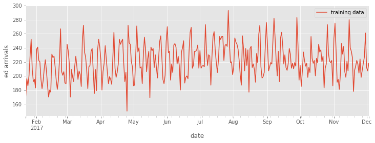
ax = train.plot(figsize=(12,4))
ax.set_ylabel('ed arrivals')
ax.legend(['training data'])

<matplotlib.legend.Legend at 0x11edfb550>

Point Forecasts

The numbers we produced using the baseline methods in the last lecture are called point forecasts. They are actually the mean value of a forecast distribution. As a reminder:

from forecast_tools.baseline import SNaive

snf = SNaive(period=7)
snf.fit(train)
preds = snf.predict(horizon=28)
preds

array([208., 218., 227., 261., 212., 207., 218., 208., 218., 227., 261.,
       212., 207., 218., 208., 218., 227., 261., 212., 207., 218., 208.,
       218., 227., 261., 212., 207., 218.])

The values in preds are point forecasts. For the time being we will focus on point forecasts. We will revisit forecast distributions in a future lecture.

Point Forecast Errors

The point forecast is our best estimate of future observations of the time series. We use our test set (some times called a holdout set) to simulate real world forecasting. As our forecasting method has not seen this data before we can measure the difference between the forecast and the ground-truth observed value.

Problem: Errors can be both positive and negative so just taking the average will mask the true size of the errors.

• There are a large number of forecast error metrics available. Each has its own pro’s and con’s. Here we review some of the most used in practice.

• forecast_tools.metrics provides a convenience function forecast_errors(y_true, y_pred, metrics='all') that quickly returns a range of the most popular error metrics as well as individual implementations.

from forecast_tools.metrics import forecast_errors, mean_absolute_error, root_mean_squared_error

errors = forecast_errors(y_true=test, y_pred=preds)
errors

{'me': -1.1428571428571428,
 'mae': 26.357142857142858,
 'mse': 1001.2244897959183,
 'rmse': 31.642131562142243,
 'mape': 12.035613307965267,
 'smape': 11.806066246602228}

errors = forecast_errors(y_true=test, y_pred=preds, metrics=['mae', 'mape'])
errors

{'mae': 26.357142857142858, 'mape': 12.035613307965267}

Calling a specific error metric function

mean_absolute_error(y_true=test, y_pred=preds)

26.357142857142858

root_mean_squared_error(y_true=test, y_pred=preds)

31.642131562142243

Comparing forecasting methods using a test (holdout) set.

Let’s compare the MAE of the methods on the ED dataset.

#convenience function for creating all objects quickly
from forecast_tools.baseline import baseline_estimators

models = baseline_estimators(seasonal_period=7)

models

{'NF1': <forecast_tools.baseline.Naive1 at 0x1a22778c10>,
 'SNaive': <forecast_tools.baseline.SNaive at 0x1a22778c90>,
 'Average': <forecast_tools.baseline.Average at 0x1a22778cd0>,
 'Drift': <forecast_tools.baseline.Drift at 0x1a22778d10>,
 'Ensemble': <forecast_tools.baseline.EnsembleNaive at 0x1a22778d50>}

HORIZON = len(test)

print(f'{HORIZON}-Step MAE\n----------')
for model_name, model in models.items():
    model.fit(train)
    preds = model.predict(HORIZON)
    mae = mean_absolute_error(y_true=test, y_pred=preds)
    print(f'{model_name}: {mae:.1f}')

28-Step MAE
----------
NF1: 23.4
SNaive: 26.4
Average: 23.7
Drift: 23.6
Ensemble: 23.6