Automating the selection of the number of replications#
sim-tools provides an implementation of the “replications algorithm” from Hoad, Robinson, & Davies (2010). Given a performance measure, and a user set CI half width precision, automatically select the number of replications.
The algorithm combines the “confidence interval” method for selecting the number of replications with a sequential look-ahead procedure to determine if a desired precision in CI is maintained given more replication.
If you make use of the code in your work please cite the GitHub repository and also the original authors article:
Hoad, Robinson, & Davies (2010). Automated selection of the number of replications for a discrete-event simulation. Journal of the Operational Research Society. https://www.jstor.org/stable/40926090
Imports#
# pylint: disable=missing-module-docstring,invalid-name
from collections.abc import Callable
from typing import Optional
import numpy as np
from treat_sim.model import Scenario, single_run
from sim_tools.output_analysis import (
ReplicationsAlgorithm,
ReplicationsAlgorithmModelAdapter,
ReplicationTabulizer,
plotly_confidence_interval_method
)
Simulation model#
We will make use of one of an example simpy models treat-sim that can be installed from PyPI
pip install treat-sim
You can read more about the model on PyPI and on the GitHub repo
The model is terminating system based on on exercise 13 from Nelson (2013) page 170.
Nelson. B.L. (2013). Foundations and methods of stochastic simulation. Springer.
from treat_sim.model import Scenario, single_run
Running a replication of the model#
To run the model you need to create an instance of Scenario. An instance of Scenario contains all of the parameters to use in the model (e.g. resources and statistical distributions for arrivals and activities). A default scenario is created like so:
scenario = Scenario()
To run a replication of the model use the single_run function. You need to pass in an instance of Scenario. The model uses common random number streams. To set the random numbers used change the random_no_set parameter
results = single_run(scenario, random_no_set=1)
print(results.T)
rep 1
00_arrivals 227.000000
01a_triage_wait 57.120114
01b_triage_util 0.621348
02a_registration_wait 90.002385
02b_registration_util 0.836685
03a_examination_wait 14.688492
03b_examination_util 0.847295
04a_treatment_wait(non_trauma) 120.245474
04b_treatment_util(non_trauma) 0.912127
05_total_time(non-trauma) 233.882040
06a_trauma_wait 133.813901
06b_trauma_util 0.834124
07a_treatment_wait(trauma) 3.715446
07b_treatment_util(trauma) 0.367507
08_total_time(trauma) 301.521195
09_throughput 161.000000
Analysing a model using a sequential algorithm#
treat-sim has been designed so that it is possible to run individual replications of the model as desired. This could be in a sequential manner as we saw above or in a batch. For example, the replications algorithm requires 3 initial replications.
The single_run function returns a pandas.DataFrame (a single row). We can access a single performance measure like so:
single_run(scenario, random_no_set=rep)["01a_triage_wait"].iloc[0]
initial_results = [
single_run(scenario, random_no_set=rep)["01a_triage_wait"].iloc[0]
for rep in range(3)
]
np.asarray(initial_results)
array([24.28094341, 57.12011429, 28.65938298])
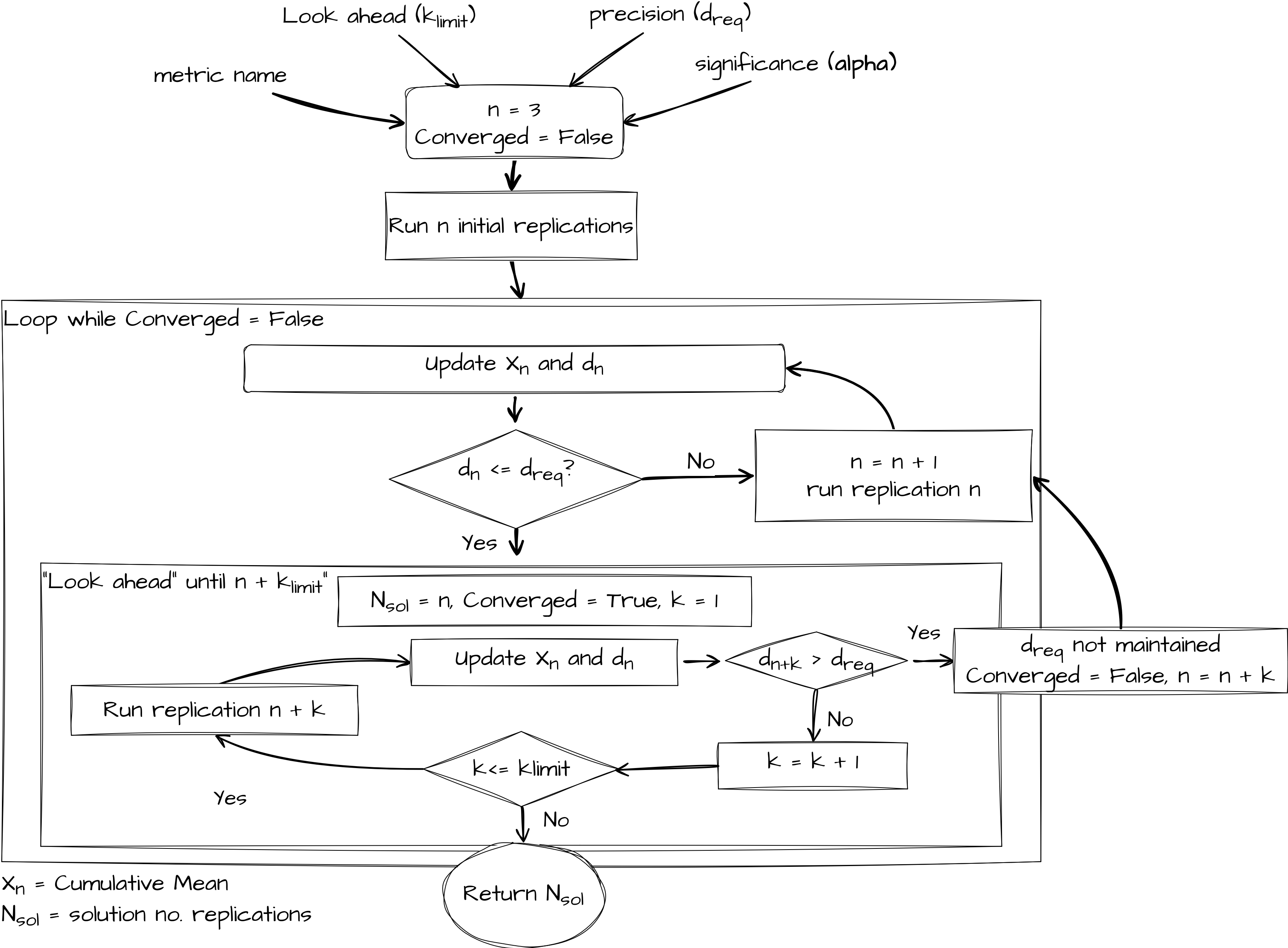
Replications Algorithm overview#
The look ahead component is governed by the formula below. A user specifies a look ahead period called \(k_{limit}\). If \(n \leq 100\) then a parameter \(k_{limit}\) is used. Hoad et al.(2010) recommend a value of 5 based on extensive empirical work. If \(n \geq 100\) then a fraction is returned. The notation \(\lfloor\) and \(\rfloor\) mean that the function must return an integer value (as it represents the number of replications to look ahead).
In general \(f(k_{limit}, n)\) means that as the number of replications increases so does the look ahead period. For example when you have run 50 replications a \(k_{limit} = 5\) means you simulate an extra 5 replications. When you have run 800 replications, a \(k_{limit} = 5\) means the number of extra replications you simulate is:
The paper provides a formal algorithm notation. Here we provide a pictorial representation of the general logic of the replications algorithm.
Adapting a simulation model to work with the ReplicationsAnalyser#
ReplicationsAnalyser has been designed to work with any Python simulation model. We know that each Python simulation model will have a slightly difference interface i.e. the setup, methods or functions to perform a single replication of the model will vary across models. ReplicationsAnalyser therefore makes use of the Adapter Pattern from Object Orientated Design principles. This means we create a “wrapper” class around the model with a known fixed interface.
We formalise Python’s duck typing feature by providing Protocol class called ReplicationsAlgorithmModelAdapter that has specifies an inteface method called single_run. The protocol is very simple i.e.
@runtime_checkable
class ReplicationsAlgorithmModelAdapter(Protocol):
"""
Adapter pattern for the "Replications Algorithm".
All models that use ReplicationsAlgorithm must provide a
single_run(replication_number) interface.
"""
def single_run(self, replication_number: int) -> float:
"""
Perform a unique replication of the model. Return a performance measure
"""
pass
For a model to use the replication algorithm it must create a concrete adapter class that implements the interface specified. Here we will create a class called TreatSimAdapter that adheres to the ReplicationsAlgorithmModelAdapter interface and pass this to the select method of a modified ReplicationsAlgorithm.
Additional imports for typing#
# pylint: disable=too-few-public-methods
class TreatSimAdapter:
"""
treat-sim single_run interface adapted for the ReplicationsAlgorithm.
"""
def __init__(
self,
scenario: Scenario,
metric: str,
single_run_func: Callable,
run_length: Optional[float] = 1140.0,
):
"""
Parameters:
------------
scenario: Scenario
The experiment and parameter class for treat-sim
metric: str
The metric to output
single_run_func: Callable
The single run function that is being adapted
run_length: float, optional (default = 1140)
The run_length for the model
"""
self.scenario = scenario
self.metric = metric
# we have passed the treat-sim single_run function as a parameter.
self.single_run_func = single_run_func
self.run_length = run_length
def single_run(self, replication_number: int) -> float:
"""
Conduct single run of the simulation.
"""
return self.single_run_func(
self.scenario,
rc_period=self.run_length,
random_no_set=replication_number,
)[self.metric].iloc[0]
Note that TreatSimAdapter does what is says on the tin: it adapts the model so that its implements the expected interface. I.e.
scenario = Scenario()
ts_model = TreatSimAdapter(scenario, "01a_triage_wait", single_run)
ts_model.single_run(1)
np.float64(57.120114285877285)
We made our Protocol runtime checkable so we can valid the interface of any models passed to the replication analyser
print(isinstance(ts_model, ReplicationsAlgorithmModelAdapter))
True
Running the ReplicationsAlgorithm#
By default the replications algorithm constructs a 95% Confidence Interval around the cumulative mean and uses a target deviation of 0.1
Optional parameters for the analyser
alpha:float, optional (default = 0.05) Used to construct the 100(1-alpha) CIhalf_width_precision:float, optional (default = 0.1) The target half width precision for the algorithm % deviation of the interval from mean.look_ahead:int, optional (default = 5) Recommended no. replications to look ahead to assess stability of precision. When the number of replications n <= 100 the value of look ahead is used. When n > 100 thenlook_ahead/ 100 * max(n, 100) is used.replication_budget:int, optional (default = 1000) A hard limit on the number of replications. Use for larger models where replication runtime is a constraint on the hardware in use.verbose:bool, optional (default=False) Display replication number as model executes.observer:ReplicationObserver| None = None Include an observer object to track how statistics change as the algorithm runs. For example,ReplicationTabulizerto return a table equivalent to confidence_interval_method.
# a default scenario
scenario = Scenario()
ts_model = TreatSimAdapter(scenario, "01a_triage_wait", single_run)
analyser = ReplicationsAlgorithm()
n_replications = analyser.select(ts_model)
print(n_replications)
145
Generating a Confidence Interval Method table#
If we wanted to track and further analyse the cumulative mean and confidence intervals of the metric analysed we can create a class that implements the ReplicationObserver interface.
@runtime_checkable
class ReplicationObserver(Protocol):
"""
Interface for an observer of an instance of the ReplicationsAnalyser
"""
def update(self, results) -> None:
"""
Add an observation of a replication
Parameters:
-----------
results: OnlineStatistic
The current replication to observe.
"""
pass
sim-tools provides a ReplicationTabulizer class that effectively returns the table used in the Confidence Interval Method as a pd.DataFrame.
scenario = Scenario()
ts_model = TreatSimAdapter(scenario, "01a_triage_wait", single_run)
observer = ReplicationTabulizer()
analyser = ReplicationsAlgorithm(observer=observer)
n_replications = analyser.select(ts_model)
observer.summary_table().head().round(2)
| Mean | Cumulative Mean | Standard Deviation | Lower Interval | Upper Interval | % deviation | |
|---|---|---|---|---|---|---|
| replications | ||||||
| 1 | 24.28 | 24.28 | NaN | NaN | NaN | NaN |
| 2 | 57.12 | 40.70 | NaN | NaN | NaN | NaN |
| 3 | 28.66 | 36.69 | 17.83 | -7.61 | 80.98 | 1.21 |
| 4 | 24.80 | 33.72 | 15.72 | 8.69 | 58.74 | 0.74 |
| 5 | 17.68 | 30.51 | 15.39 | 11.40 | 49.62 | 0.63 |
You can visualise the tabulized results using the plotly_confidence_interval_method function.
plotly_confidence_interval_method(n_replications, observer.summary_table(),
"01a_triage_wait")