Time dependent arrivals via thinning#
This notebook provides an overview of how to use the time_dependent.NSPPThinning class.
Thinning is an acceptance-rejection approach to sampling inter-arrival times (IAT) from a time dependent distribution where each time period follows its own exponential distribution.
There are two random variables employed in sampling: an exponential distribution (used to sample IAT) and a uniform distibution (used to accept/reject samples).
All IATs are sampled from an Exponential distribution with the highest arrival rate (most frequent). These arrivals are then rejected (thinned) proportional to the ratio of the current arrival rate to the maximum arrival rate. The algorithm executes until a sample is accepted. The IAT returned is the sum of all the IATs that were sampled.
The thinning algorithm#
A NSPP has arrival rate $\lambda(t)$ where $0 \leq t \leq T$
Here $i$ is the arrival number and $\mathcal{T_i}$ is its arrival time.
Let $\lambda^* = \max_{0 \leq t \leq T}\lambda(t)$ be the maximum of the arrival rate function and set $t = 0$ and $i=1$
Generate $e$ from the exponential distribution with rate $\lambda^*$ and let $t = t + e$ (this is the time of the next entity will arrive)
Generate $u$ from the $U(0,1)$ distribution. If $u \leq \dfrac{\lambda(t)}{\lambda^*}$ then $\mathcal{T_i} =t$ and $i = i + 1$
Go to Step 2.
sim-tools imports#
from sim_tools.datasets import load_banks_et_al_nspp
from sim_tools.time_dependent import NSPPThinning, nspp_plot, nspp_simulation
# general imports
import matplotlib.pyplot as plt

# ggplot style for plots
plt.style.use("ggplot")
Example from Banks et al.#
We will illustrate the use of NSPPThinning using an example from Banks et al.
The table below breaks an arrival process down into 60 minutes intervals.
t(min) |
Mean time between arrivals (min) |
Arrival Rate $\lambda(t)$ (arrivals/min) |
|---|---|---|
0 |
15 |
1/15 |
60 |
12 |
1/12 |
120 |
7 |
1/7 |
180 |
5 |
1/5 |
240 |
8 |
1/8 |
300 |
10 |
1/10 |
360 |
15 |
1/15 |
420 |
20 |
1/20 |
480 |
20 |
1/20 |
Interpretation: In the table above the fastest arrival rate is 1/5 customers per minute or 5 minutes between customer arrivals.
data = load_banks_et_al_nspp()
data
| t | mean_iat | arrival_rate | |
|---|---|---|---|
| 0 | 0 | 15 | 0.066667 |
| 1 | 60 | 12 | 0.083333 |
| 2 | 120 | 7 | 0.142857 |
| 3 | 180 | 5 | 0.200000 |
| 4 | 240 | 8 | 0.125000 |
| 5 | 300 | 10 | 0.100000 |
| 6 | 360 | 15 | 0.066667 |
| 7 | 420 | 20 | 0.050000 |
| 8 | 480 | 20 | 0.050000 |
# create arrivals and set random number seeds
SEED_1 = 42
SEED_2 = 101
arrivals = NSPPThinning(data, SEED_1, SEED_2)

# number of arrivals to simulate
n_arrivals = 15

# run simulation
simulation_time = 0.0
for _ in range(n_arrivals):
    iat = arrivals.sample(simulation_time)
    simulation_time += iat
    print(f"{simulation_time:.2f} Patient arrival (IAT={iat:.2f})")
37.46 Patient arrival (IAT=37.46)
73.02 Patient arrival (IAT=35.56)
89.41 Patient arrival (IAT=16.39)
96.79 Patient arrival (IAT=7.38)
98.37 Patient arrival (IAT=1.58)
104.94 Patient arrival (IAT=6.57)
112.30 Patient arrival (IAT=7.35)
121.49 Patient arrival (IAT=9.19)
127.62 Patient arrival (IAT=6.14)
135.25 Patient arrival (IAT=7.63)
135.64 Patient arrival (IAT=0.39)
141.91 Patient arrival (IAT=6.27)
148.23 Patient arrival (IAT=6.32)
155.26 Patient arrival (IAT=7.04)
158.47 Patient arrival (IAT=3.21)
Check NSPP is working as expected#
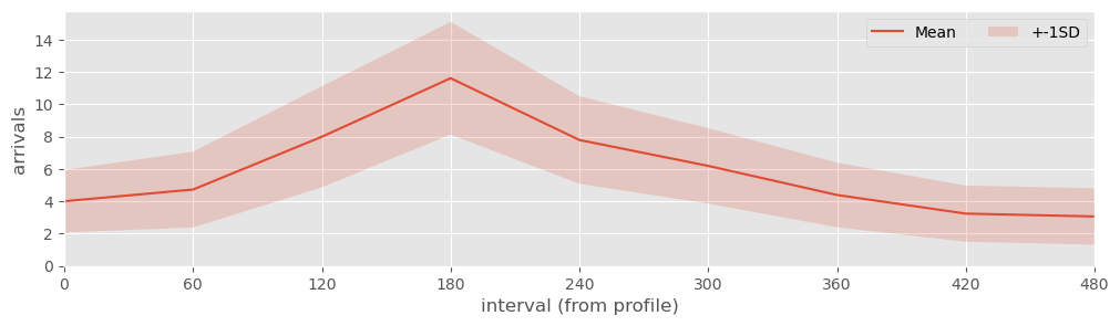
As part of model testing you can check that the NSPP for arrivals has been setup correctly by using nspp_plot. This runs multiple replications of the NSPP and returns a plot of the number of arrivals per interval. The profile can be used as a sense check. If you prefer to have the data in tabular form you can use nspp_simulation that returns a pd.DataFrame containing multiple replications of the number of arrivals per interval.
NSPP plot#
fig, ax = nspp_plot(data, run_length=540)
Tabular NSPP data#
The function nspp_simulation returns a pd.DataFrame. By default 1000 replications of the NSPP are run. The run length can be specified, but if omitted it defaults to the last interval + interval width in the arrival profile.
In the Banks et al. example we are given the rate per minute of arrivals. We therefore multiply this by 60 get the expected number of arrivals in an hour. We compare this to the actual simulated.
nspp_replications = nspp_simulation(data, n_reps=1000)

# peak at data
nspp_replications.head()
| 0 | 1 | 2 | 3 | 4 | 5 | 6 | 7 | 8 | |
|---|---|---|---|---|---|---|---|---|---|
| rep | |||||||||
| 1 | 1 | 5 | 7 | 13 | 9 | 11 | 5 | 3 | 1 |
| 2 | 6 | 7 | 4 | 9 | 6 | 8 | 5 | 1 | 3 |
| 3 | 3 | 2 | 6 | 13 | 4 | 6 | 2 | 1 | 5 |
| 4 | 4 | 2 | 8 | 10 | 7 | 7 | 5 | 1 | 9 |
| 5 | 2 | 4 | 10 | 13 | 10 | 7 | 8 | 4 | 5 |
# re-label columns
nspp_replications.columns = data["t"].values


## banks data converted from arrivasl per min to arrivals per hour
data["expected_mean_arrivals_hr"] = data["arrival_rate"] * 60.0
data["simulated_mean_arrivals_hr"] = nspp_replications.mean(axis=0).values
data.round(1)
| t | mean_iat | arrival_rate | expected_mean_arrivals_hr | simulated_mean_arrivals_hr | |
|---|---|---|---|---|---|
| 0 | 0 | 15 | 0.1 | 4.0 | 4.0 |
| 1 | 60 | 12 | 0.1 | 5.0 | 4.7 |
| 2 | 120 | 7 | 0.1 | 8.6 | 8.0 |
| 3 | 180 | 5 | 0.2 | 12.0 | 11.6 |
| 4 | 240 | 8 | 0.1 | 7.5 | 7.8 |
| 5 | 300 | 10 | 0.1 | 6.0 | 6.2 |
| 6 | 360 | 15 | 0.1 | 4.0 | 4.4 |
| 7 | 420 | 20 | 0.0 | 3.0 | 3.2 |
| 8 | 480 | 20 | 0.0 | 3.0 | 3.1 |